How-To

How to Use Filters in Microsoft Excel to Find Data Faster

By Sandy Writtenhouse

Updated January 21, 2021

Learn how to apply filters in Excel to make analyzing your data easier. You can filter by color, condition, or value to find data fast.

Microsoft Excel is a full-featured spreadsheet application with helpful features to ease the task of data analysis. You can create a pivot table to find data trends and make a pie chart to visually analyze data sets.

But what if you just need a simple way to locate specific data? Filters in Excel give you easy ways to find the data you want. Especially useful in data-heavy spreadsheets, filters can be quickly applied and just as easily removed when you’re finished with them.

Data for Filters in Excel

Filters in Excel apply to columns. This doesn’t mean that you can’t use a filter if you don’t include an entire column. Just note that with whatever data set you select; the filter will be placed at the tops of the columns for the selected cells. Here’s a visual example.

You can see only a subset of data selected (D9:F13). When the filter is applied, the filter indicators (arrows) are at the top of the columns within that data set. And the only data available to filter is in the cells beneath.

Also, you can apply filters only to adjacent cells – a single cell range. If you try to select multiple cell ranges, you’ll receive an error.

Turn on the Filter

If you’re ready to apply a filter, select the data you want to use keeping the above points in mind. Simply drag through the cell range. Then, click the Data tab and hit the Filter button in the ribbon.

You’ll immediately see the filter arrows in the selected columns. Once you actually apply a filter, you’ll notice a small filter image next to the indicator for the corresponding column. So if you forget that you have a filter applied or don’t remember where you set it, this is your signal.

Apply a Filter in Excel

The next step in the process is to apply a filter. If you really want to narrow down the data, you can use more than one filter in the data set, meaning in more than one column. For the purposes of this how-to, we’ll stick with one filter.

Select the arrow next to the column you want to filter. In the pop-up window, you’ll notice that you have sort options at the top. So keep this in mind too, if you want to change the order of your data.

You can filter by color, condition, or value. Let’s look at an example of each.

Filter by Color

If you use a feature like conditional formatting in Excel, a color filter is a terrific tool. And you can choose to use the color of a cell or the text.

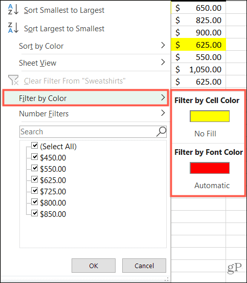
In this example, we have cells highlighted in our sheet and want to pull them all together to analyze the data.

1. Select the filter arrow for the column.
2. Move your cursor to Filter by Color.
3. Choose the color filter you want to use in the pop-out menu. Excel is smart enough to know when you have cell or text colors in the data you’re filtering.
4. Click OK.

Filter by Condition

Just like Excel knows when you use colors, it knows the types of data in your set. So you can filter by a condition for numbers, text, or dates. And the one of those three that appears in the menu corresponds to the type of data and the condition options.

In this example, we have numbers (currency) that we want to filter for a closer look.

1. Select the filter arrow for the column.
2. Move your cursor to Numbers Filters (or, Date Filters or Text Filters depending on your data type).
3. Choose the condition you want to use in the pop-out menu. For Numbers you have options like Equals, Greater Than, and Above Average.
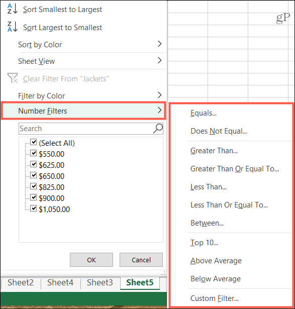
4. Depending on the condition you choose in Step 3, you may see a pop-up window to enter additional details. For instance, if you use the Numbers Filter and pick Equals as the condition, you’ll enter the “equals to” value in the window.
5. Click OK.

Filter by Value

One of the quickest filters in the list is value. At the bottom of the filter window, you’ll see all the values in that column of your data set. Use the checkboxes to select the value(s) for the filter and click OK.

If the data set contains many values, you can speed up finding the one you want by using the Search box directly above it. Just enter the number, date, or text and your results display with that item’s box checked. Click OK to apply the filter.

Remove a Filter

Once you apply a filter in Excel, it will remain until you remove it. And you can remove a filter in two different ways.

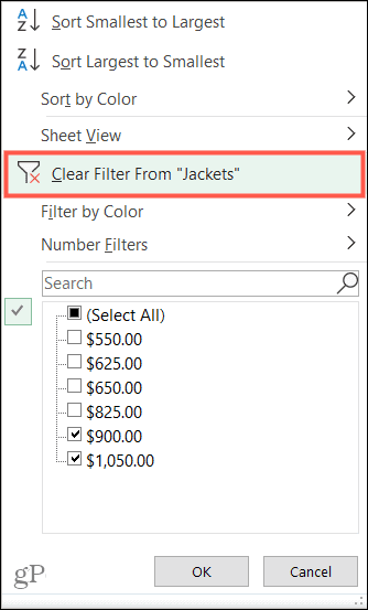
If you only want to remove a single filter, click the filter arrow and select Clear Filter From [Data].

If you want to remove all filters you’ve applied to a sheet, head to the Data tab and turn off the Filter button.

Find Your Data Faster with Filters in Excel

By using filters in Excel, you can quickly spot the data you want. Whether you need data for products with a certain color, payees with a specific dollar amount, or dates when you ordered items, filters in Excel can help you find it fast!

If you’re also interested in quicker ways to enter data before you analyze it, check out our how-tos for using autofill in Excel and creating a data entry form.