How-To

How to Use SUMIF Function in Google Sheets

By Adam Davidson

Published May 16, 2022

Google Sheets has more than 400 functions, including the useful SUMIF function, which you can use for advanced calculations. Here’s how to use it.

Google Sheets includes a number of powerful functions. These functions allow you to create formulas that you can use to manipulate data or calculate values in your spreadsheet.

One of the most useful functions is SUMIF. Similar to the basic SUM function, this allows you to find the total of a set of values. What makes SUMIF different is that it will only include values that meet a specific criterion that you set.

If you want to know how to use the SUMIF function in Google Sheets, follow our guide below.

What is the SUMIF Function in Google Sheets?

The SUMIF function in Google Sheets is a simple but effective function that allows you to sum multiple cells from your data, provided that they meet a specific criterion.

For example, if you have a list of sales figures, and you wanted to know how much money you’d made from higher ticket items, you might use this function to sum the total value of sales from items that cost $500 or more.

The syntax of the formula is as follows:

SUMIF(range, criterion, [sum_range])

The range is the selection of cells that you want the function to examine. The criterion is the condition that a cell must meet for its value to be included in the sum. The sum range is in square brackets, indicating that this is an optional argument that does not need to be included in the function.

You can use the sum range if you want to sum the values from a different column. For example, instead of summing the value of items that cost more than $500, you could sum the column that holds the number of sales, to find out how many items above this value you’ve sold.

How to Use the SUMIF Function in Google Sheets Within the Given Range

If you want to sum the values within your given range, you’ll only need to enter two values into your function.

Here’s how to use the SUMIF function within your given range:

1. Click in the cell where you want the function to appear.
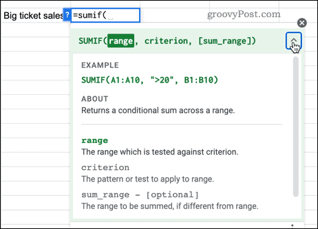
2. Type =SUMIF( and you’ll see the function information appear beneath the cell.
   
3. You can click on the down arrow for more information about how the function works.
   
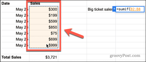
4. Select the cells that you want the function to apply to (or type the cell range manually).
   
5. Click back into your function and type a comma.
   
6. Enter your criterion in quotes, followed by a closed bracket. Your criterion could be a value, text, a logical expression, or even another function.
   
7. Hit Enter and your function will calculate, with the output showing in the cell.
   

In this example, the function has found all of the items that were sold for more than $500 and found the total of all those sales.

How to Use the SUMIF Function in Google Sheets With a Different Range

Sometimes you may want to search for values that meet a specific criterion but then want to sum other values from the same row. For example, for all sales over $500, you might want to sum the total number of products sold, rather than their sale price.

Here’s how to use the SUMIF function with a different range:

1. Click in the cell where you want the function to appear.
2. Type =SUMIF( and you’ll see the function information appear beneath the cell.
   
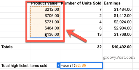
3. Now highlight the cells that you want the function to apply to.
   
4. Click back into your function, and type a comma.
   
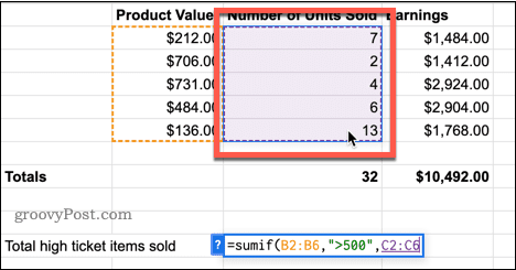
5. Enter your criterion in quotes and type another comma.
   
6. Select the cells that you want to sum (or type the range in manually).
   
7. Type a final closed bracket and hit Enter.
   
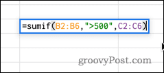
8. Your function will now calculate, with the output showing in the cell.
   

Make the Most of Google Sheets Functions

Google Sheets has almost 500 different functions, covering everything from statistics to text manipulation. The more functions you know about, the more powerful Google Sheets becomes.

Google Sheets IF statements are an effective way to add multiple criteria to your functions. The SORT function allows you to alphabetize your Google Sheets data. You can even use a function (GOOGLEFINANCE) to track stocks in Google Sheets.